I post the code I wrote in various projects here for reference. If there is any problem or advice, feel free to contact me at my email (jing.zhang17@case.edu).
Synthetic data (Download) is used to illustrate results. Some data may not be meaningful.
There are 159 observations, 64 of which are in Group0, the control group, and 95 of which are in Group1, the experiment group.
The 20 variables are as follows.
| Variable name | Notes |
|---|---|
| id | identity number |
| group | in Group0 or Group1 |
| age | continuous variable |
| agegroup | discrete variable |
| bmi | body mass index, continuous variable |
| sex | discrete variable |
| ecog | Eastern Cooperative Oncology Group performance, discrete variable |
| stage | cancer stage, discrete variable |
| class | cancer classification, discrete variable |
| week | treatment duration in weeks, continuous variable |
| cycle | number of treatment cycles |
| dose | dose intensity % |
| totaldose | total cumulative dose mg |
| pfsyear | progression-free survival in years |
| pfscensor | progression-free censor with 0 equaling to censored and 1 equaling to event |
| response | types of status which include complete response, partial response, stable disease and progressive disease |
| doryear | duration of response for patients with complete or partial response |
| dorcensor | duration of response censor with 0 equaling to censored and 1 equaling to event |
| adverse1 | grade of adverse event 1, such as nausea, with 0 equaling to not experiencing adverse event 1 |
| adverse2 | grade of adverse event 1, such as nausea, with 0 equaling to not experiencing adverse event 1 |
dt<-read.csv("https://jingzhang1.github.io/assets/clinical%20trial%20project/example_data.csv")
head(dt)
##       id group age agegroup  bmi sex ecog stage class week cycle dose
## 1 688265     0  61        1 20.6   1    0     2     1 87.7     2 84.8
## 2 691261     0  44        1 21.2   1    1     2     1 93.2     2 80.6
## 3 754859     0  71        2 20.2   1    0     2     2 78.4     2 74.1
## 4 687411     0  56        1 26.7   1    2     2     1 68.0     2 52.7
## 5 689438     0  73        2 22.0   1    2     2     1 90.3     2 89.9
## 6 670733     0  60        1 20.7   2    0     2     1 67.8     2 86.9
##   totaldose pfsyear pfscensor response doryear dorcensor adverse1 adverse2
## 1      1696     4.6         1        3      NA        NA        1        0
## 2      1612     4.6         1        3      NA        NA        1        0
## 3      1482     2.8         1        3      NA        NA        1        2
## 4      1054     4.7         1        3      NA        NA        2        2
## 5      1798     1.5         0        3      NA        NA        0        3
## 6      1738     5.2         1        3      NA        NA        2        1
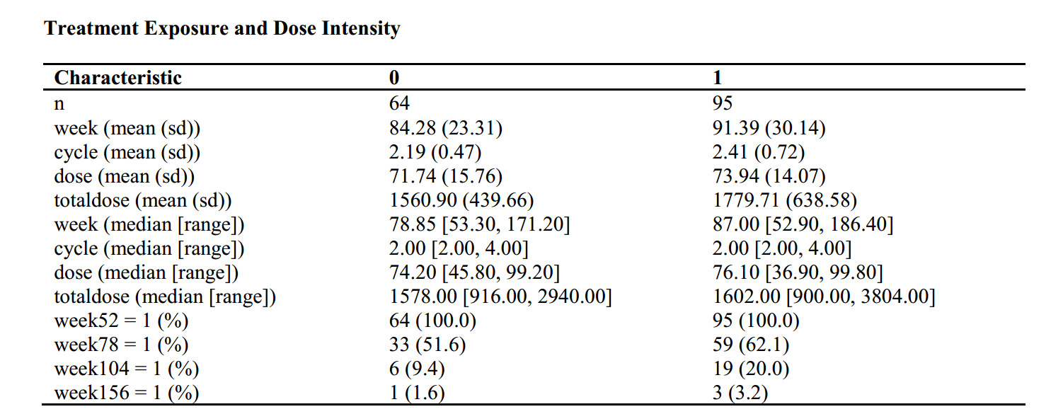
library("tableone")
listVars<-c("week","cycle","dose","totaldose")
table1 <- CreateContTable(vars = listVars, data = dt,strata = "group", test = F)
###mean sd
table2 <- print(table1,quote = F,varLabels = T,printToggle=F, noSpaces = TRUE)
table2<-as.data.frame(table2)
###median range
table3 <- print(table1,nonnormal =listVars,minMax=T,quote = F,varLabels = T,printToggle=F,  noSpaces = TRUE)
table3<-as.data.frame(table3)

###week proportion
#cutoff:52,78,104,156
dt$week52<-ifelse(dt$week>52,1,0)
dt$week78<-ifelse(dt$week>78,1,0)
dt$week104<-ifelse(dt$week>104,1,0)
dt$week156<-ifelse(dt$week>156,1,0)
listVars<-c("week52","week78","week104","week156")
table4 <- CreateCatTable(vars = listVars, data = dt,strata = "group", test = F,includeNA=T)
table5<-print(table4,showAllLevels = F,quote = F,varLabels = T,printToggle=F, noSpaces = TRUE)
table5<-as.data.frame(table5)

tablesum<-rbind(table2,table3[-1,],table5[-1,])

# Write to RTF files
library(dplyr)
tablesum <- tablesum %>%
  mutate(Characteristic = rownames(.)) %>%
  select(Characteristic, everything()) %>%
  mutate_all(trimws)
library(rtf)
rtffile <- RTF("Treatment Exposure and Dose Intensity.rtf")
addHeader(rtffile, "Treatment Exposure and Dose Intensity")
#addParagraph(rtffile, "Ouput for table:\n")
addTable(rtffile, tablesum, NA.string="")
done(rtffile)
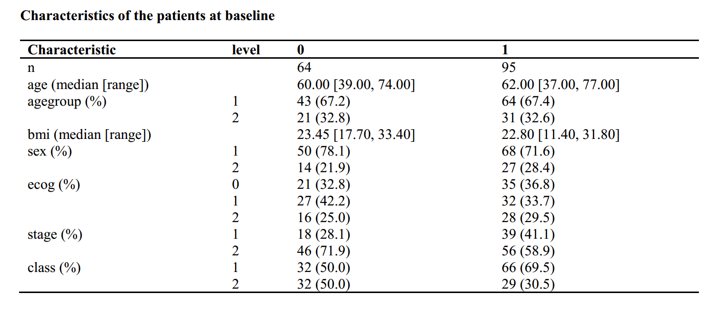
library("tableone")
listVars <- c("age","agegroup","bmi","sex","ecog","stage","class")
factorVars<-c("agegroup","sex","ecog","stage","class")
table1 <- CreateTableOne(vars = listVars, data = dt, factorVars = factorVars,strata = "group",test=F)
###mean sd
table2 <- print(table1, showAllLevels = TRUE,quote = F,varLabels = T,printToggle=F, noSpaces = TRUE)
table2<-as.data.frame(table2)
###median range
table3 <- print(table1, showAllLevels = TRUE,quote = F,varLabels = T,nonnormal=c("age","bmi"), minMax=T, printToggle=F, noSpaces = TRUE)
table3<-as.data.frame(table3)

# Write to RTF files
library(dplyr)
table3 <- table3 %>%
  mutate(Characteristic = rownames(.)) %>%
  select(Characteristic, everything()) %>%
  mutate_all(trimws)
library(rtf)
rtffile <- RTF("Characteristics of the patients at baseline.rtf")
addHeader(rtffile, "Characteristics of the patients at baseline")
addTable(rtffile, table3, NA.string="")
done(rtffile)
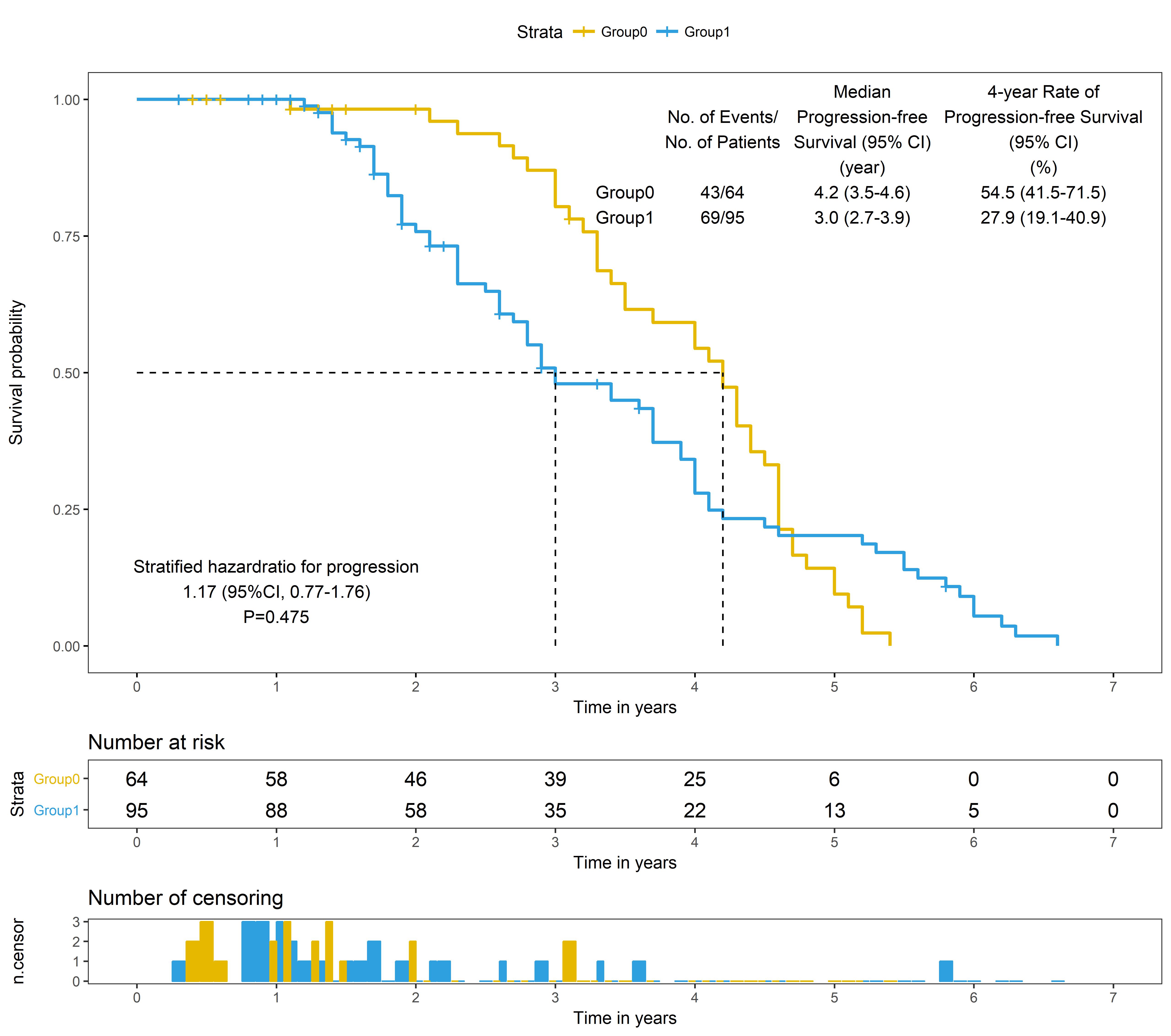
library("survival")
library("survminer")
fit <- survfit(Surv(pfsyear, pfscensor) ~ group, data = dt)
km<-ggsurvplot(fit,                     # survfit object with calculated statistics.
           censor=T,
           pval = F,                    # show p-value of log-rank test.
           conf.int = F,                # show confidence intervals for point estimaes of survival curves.
           surv.median.line = "hv",     # add the median survival pointer.
           xlim=c(0,7),
           xlab = "Time in years",      # customize X axis label.
           break.time.by = 1,           # break X axis in time intervals by 200.
           risk.table = "absolute",     # absolute number and percentage at risk.
           risk.table.y.text.col = T,   # colour risk table text annotations.
           risk.table.y.text = T,       # show bars instead of names in text annotations in legend of risk table.
           ncensor.plot = TRUE,         # plot the number of censored subjects at time t
           legend.labs =c("Group0", "Group1"),
           palette =c("#E7B800", "#2E9FDF"),
           ggtheme =theme_bw()+theme(plot.background = element_blank(),
                                     panel.grid.major = element_blank(),
                                     panel.grid.minor = element_blank())
)

###stratified cox model HR
model<-coxph(Surv(pfsyear,pfscensor)~group+strata(stage,class),data=dt)
a<-summary(model)
hrci<-paste(round(a$conf.int[1],2)," (95%CI, ",round(a$conf.int[3],2),"-",round(a$conf.int[4],2),")",sep="")

###stratified log rank
survdiff(Surv(pfsyear, pfscensor) ~ group + strata(stage,class), data=dt, rho = 0 )#0.475
p<-"P=0.475"

###Summary of survival
summary(fit)
summary(fit)$table
text0<-paste(paste(" "," "," "," ",sep  = "\n"),"Group0","Group1",sep  = "\n")
text1<-paste(paste(" ","No. of Events/","No. of Patients"," ",sep  = "\n"),"43/64","69/95",sep  = "\n")
text2<-paste(paste("Median", "Progression-free", "Survival (95% CI)","(year)",sep  = "\n"),"4.2 (3.5-4.6)","3.0 (2.7-3.9)",sep  = "\n")
text3<-paste(paste("4-year Rate of", "Progression-free Survival", "(95% CI)","(%)",sep  = "\n"),"54.5 (41.5-71.5)","27.9 (19.1-40.9)",sep  = "\n")
cat(text1)
cat(text2)
cat(text3)
km$plot<-km$plot+annotate("text", x=1, y=0.1,label=paste("Stratified hazardratio for progression",hrci,p,sep  = "\n"))+
  annotate("text", x=3.5, y=0.9,label=text0)+
  annotate("text", x=4.2, y=0.9,label=text1)+
  annotate("text", x=5.2, y=0.9,label=text2)+
  annotate("text", x=6.5, y=0.9,label=text3)

km1<-list()
km1[[1]]<-km
km2<-arrange_ggsurvplots(km1, print = F,ncol = 1, nrow = 1,
                         surv.plot.height=0.7,
                         risk.table.height = 0.15,
                         ncensor.plot.height =0.15)
ggsave(filename="Kaplan-Meier plot.jpeg", km2, width=26, height=23, dpi=500, units="cm")
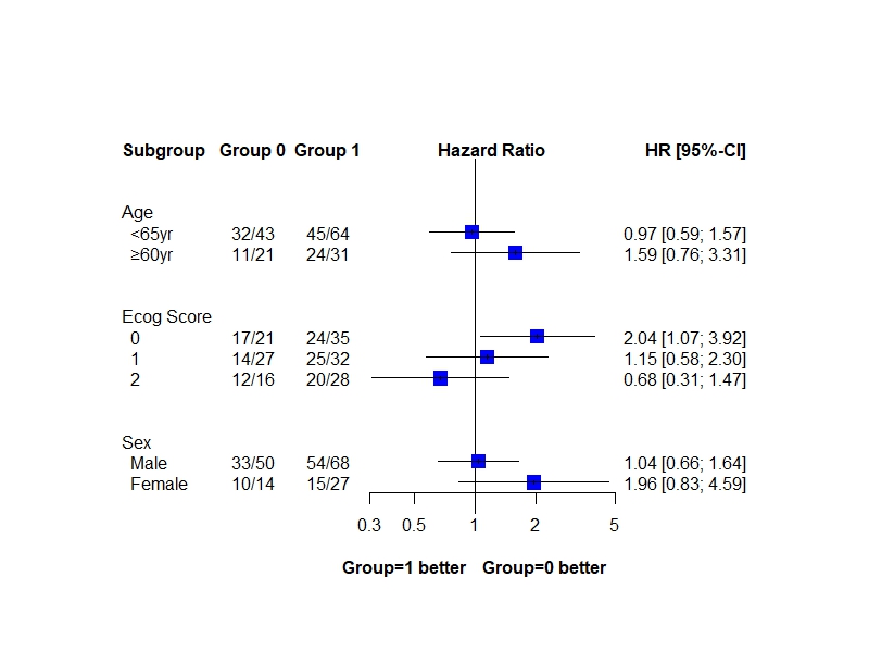
library("survival")
sex1<-coxph(Surv(pfsyear,pfscensor)~group,subset={sex==1},data=dt)
sex2<-coxph(Surv(pfsyear,pfscensor)~group,subset={sex==2},data=dt)

ageg1<-coxph(Surv(pfsyear,pfscensor)~group,subset={agegroup==1},data=dt)
ageg2<-coxph(Surv(pfsyear,pfscensor)~group,subset={agegroup==2},data=dt)

ecog0<-coxph(Surv(pfsyear,pfscensor)~group,subset={ecog==0},data=dt)
ecog1<-coxph(Surv(pfsyear,pfscensor)~group,subset={ecog==1},data=dt)
ecog2<-coxph(Surv(pfsyear,pfscensor)~group,subset={ecog==2},data=dt)


coef<-c(0.0366,0.672,-0.0353,0.463,0.715,0.141,-0.393)  ##coefficient in cox (not HR)
se<-c(0.2334,0.435,0.2492,0.374,0.332,0.354,0.398)  ##se(coef) in cox

datacoef<-data.frame(group=c("Sex","  Male","  Female","Age","  <65yr","  ≥60yr","Ecog Score","  0","  1","  2"),
                   coef=c(NA,0.0366,0.672,NA,-0.0353,0.463,NA,0.715,0.141,-0.393),
                   se=c(NA,0.2334,0.435,NA,0.2492,0.374,NA,0.332,0.354,0.398),
                   subgroup=c("Sex","Sex","Sex","Age","Age","Age","Ecog Score","Ecog Score","Ecog Score","Ecog Score"))

###no.death/no.total
addmargins(xtabs(~sex+pfscensor+group,data=dt))
addmargins(xtabs(~agegroup+pfscensor+group,data=dt))
addmargins(xtabs(~ecog+pfscensor+group,data=dt))

grp0<-c("","33/50","10/14", "","32/43","11/21", "","17/21","14/27","12/16")
grp1<-c("","54/68","15/27", "","45/64","24/31", "","24/35","25/32","20/28")

datacoef<-cbind(datacoef,grp0,grp1)

library(meta)
metaba<-metagen(coef,se,data=datacoef,sm="HR",studlab=group,
                label.e="group=0",label.c="group=1",
                byvar=subgroup,print.byvar = TRUE)
plot<-forest(metaba,
       leftcols=c("group","grp0","grp1"),
       leftlabs=c("Subgroup", "Group 0", "Group 1"),
       just.addcols.left=c("left","center","center"),
       rightcols=c("effect.ci"),
       col.square="blue",
       squaresize=0.7,
       xlim=c(0.3, 5),
       label.right="Group=0 better", col.label.right="black",
       label.left="Group=1 better", col.label.left="black",
       ff.lr="bold",
       weight.study="same",
       ref=1,print.I2=FALSE,print.tau2=FALSE,
       comb.fixed=FALSE,print.Q.subgroup=FALSE,comb.random=FALSE)
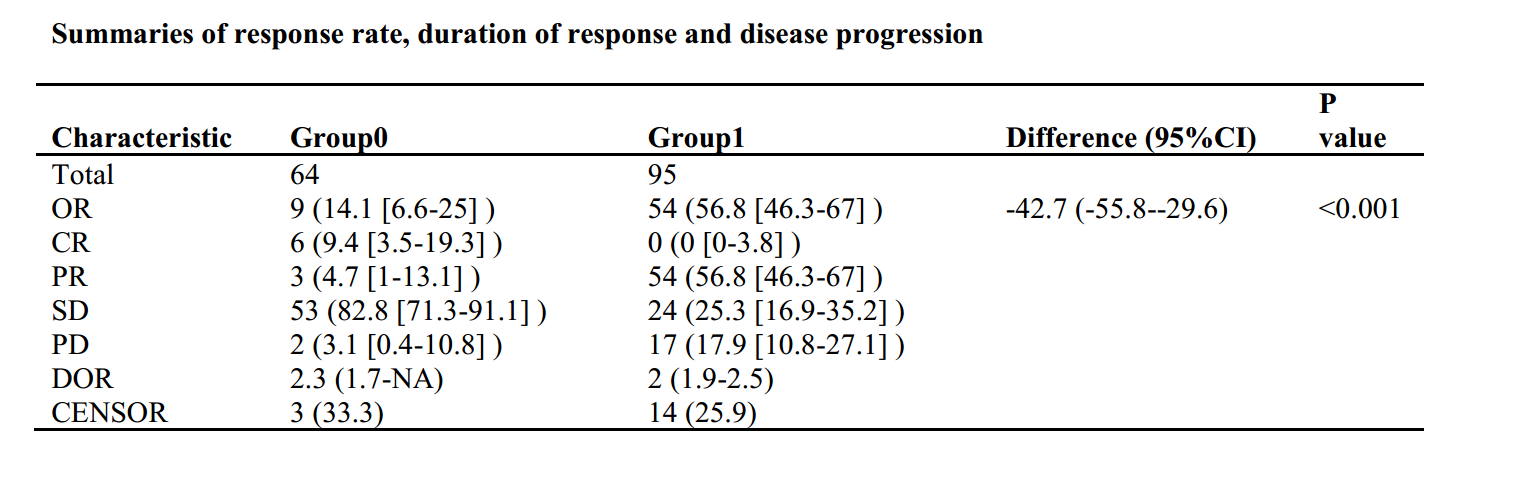
library("tableone")
table1 <- CreateCatTable(vars = "response", data = dt, strata = "group",test=F)
table2 <- print(table1, showAllLevels = TRUE,quote = F,varLabels = T,format = "f")
table2<-as.data.frame(table2)
table2<-table2[,-1]
rownames(table2)<-c("Total","CR","PR","SD","PD")
colnames(table2)<-c("Group0","Group1")
table2$Group0<-as.numeric(as.character(table2$Group0))
table2$Group1<-as.numeric(as.character(table2$Group1))
table2["OR",1]<-table2["CR",1]+table2["PR",1]
table2["OR",2]<-table2["CR",2]+table2["PR",2]

table2[,c(3:8)]<-NA
for (i in 1:5){
  for (j in 1:2){
    table2[i+1,j+2]<-round(table2[i+1,j]/table2[1,j]*100,1)
    table2[i+1,j+4]<-round(binom.test(table2[i+1,j], table2[1,j])$conf.int[1]*100,1) #Clopper and Pearson
    table2[i+1,j+6]<-round(binom.test(table2[i+1,j], table2[1,j])$conf.int[2]*100,1)
  }
}

table2[,c(9:10)]<-NA
for (i in 1:5){
  for (j in 1:2){
    table2[i+1,j+8]<-paste(table2[i+1,j]," (",table2[i+1,j+2]," [",table2[i+1,j+4],"-",table2[i+1,j+6],"] )",sep="")
  }
}
table2[1,9]<-table2[1,1]
table2[1,10]<-table2[1,2]
table2[,c(1:8)]<-NULL

###DOR,CENSOR
library("survival")
fitdor <- survfit(Surv(doryear, dorcensor) ~ group, data = dt)
dorsum<-summary(fitdor)$table

for (i in 1:2){
  table2["DOR",i]<-paste(dorsum[i,"median"]," (",dorsum[i,"0.95LCL"],"-",dorsum[i,"0.95UCL"],")",sep="")
  table2["CENSOR",i]<-paste(dorsum[i,"records"]-dorsum[i,"events"]," (",
                            round((dorsum[i,"records"]-dorsum[i,"events"])/dorsum[i,"records"]*100,1),")",sep="")
}

table2<-table2[c("Total","OR","CR","PR","SD","PD","DOR","CENSOR"),]

dt$response1<-ifelse(dt$response<3,1,ifelse(dt$response>2,2,NA))
dt$strata<-interaction(dt$stage,dt$class)
mytable <- xtabs(~group+response1+strata, data=dt)
a<-mantelhaen.test(mytable)
a$p.value

addmargins(table(dt$response1,dt$group),1)
prop.table(table(dt$response1,dt$group),2)
ord<-0.141-0.568
ordse<-sqrt(0.141*(1-0.141)/64+0.568*(1-0.568)/95)
ordlow<-round(ord-1.96*ordse,3)
ordup<-round(ord+1.96*ordse,3)

table2[2,3]<-paste(ord*100," (",ordlow*100,"-",ordup*100,")",sep="")
table2[2,4]<-ifelse(a$p.value<0.001,"<0.001",round(a$p.value,3))
colnames(table2)<-c("Group0","Group1","Difference (95%CI)","P value")

# Write to RTF files
library(dplyr)
table2 <- table2 %>%
  mutate(Characteristic = rownames(.)) %>%
  select(Characteristic, everything()) %>%
  mutate_all(trimws)
library(rtf)
rtffile <- RTF("Summaries of response rate, duration of response and disease progression.rtf")
addHeader(rtffile, "Summaries of response rate, duration of response and disease progression")
addTable(rtffile, table2,NA.string="")
done(rtffile)
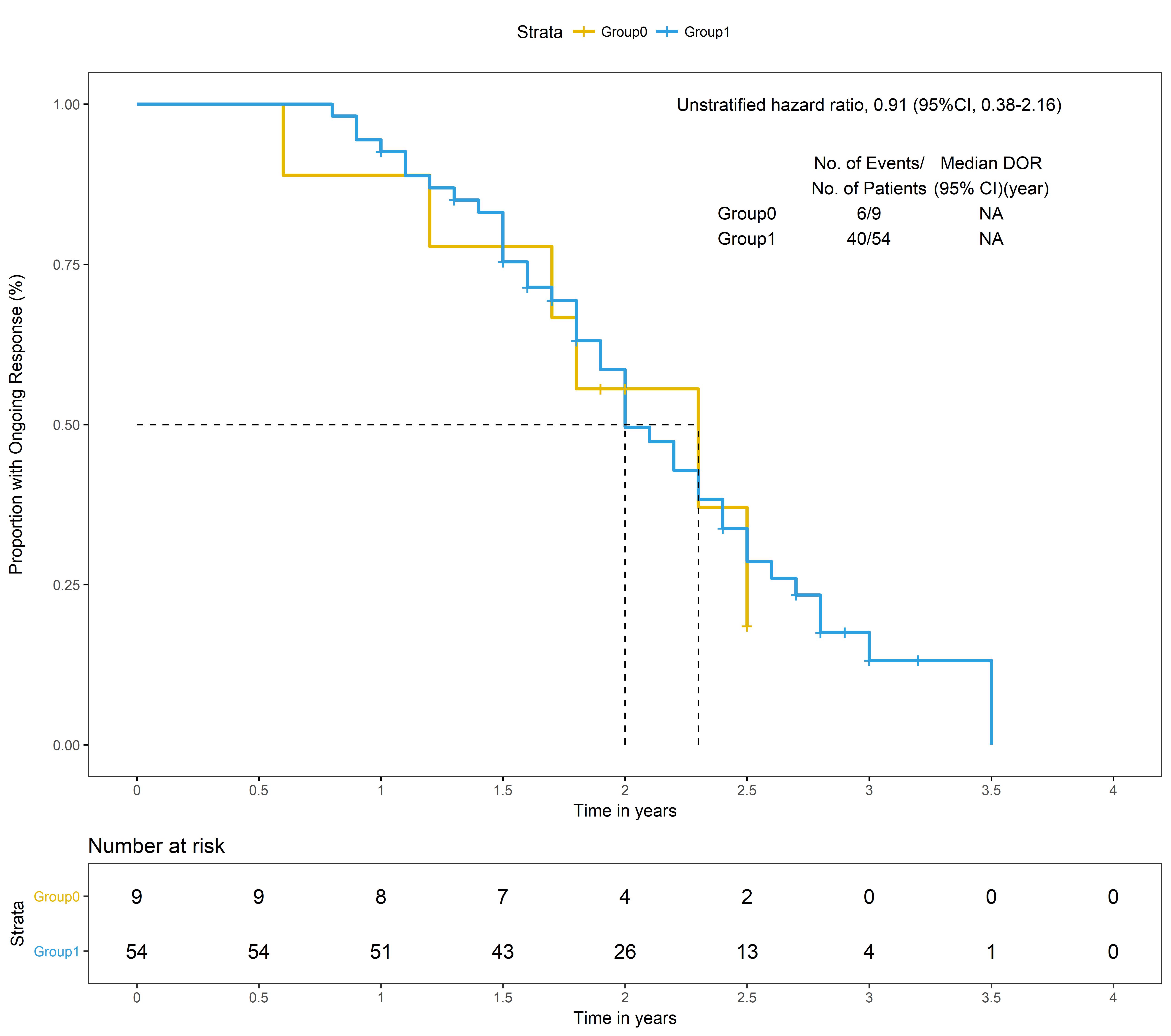
library("survival")
library("survminer")
fitdor <- survfit(Surv(doryear, dorcensor) ~ group, data = dt)
dor<-ggsurvplot(fitdor,                     # survfit object with calculated statistics.
               censor=T,
               pval = F,                    # show p-value of log-rank test.
               conf.int = F,                # show confidence intervals for point estimaes of survival curves.
               surv.median.line = "hv",     # add the median survival pointer.
               xlim=c(0,4),
               xlab = "Time in years",      # customize X axis label.
               ylab="Proportion with Ongoing Response (%)",
               break.time.by = 0.5,         # break X axis in time intervals by 200.
               risk.table = "absolute",     # absolute number and percentage at risk.
               ncensor.plot = F,            # plot the number of censored subjects at time t
               legend.labs =c("Group0", "Group1"),
               palette =c("#E7B800", "#2E9FDF"),
               ggtheme =theme_bw()+theme(plot.background = element_blank(),
                                         panel.grid.major = element_blank(),
                                         panel.grid.minor = element_blank())
)
###unstratified cox model HR
model<-coxph(Surv(doryear,dorcensor)~group,data=dt)
a<-summary(model)
hrci<-paste(round(a$conf.int[1],2)," (95%CI, ", round(a$conf.int[3],2), "-", round(a$conf.int[4],2),")", sep="")

dorsum<-summary(fitdor)$table
text0<-paste(paste(" "," ",sep  = "\n"),"Group0","Group1",sep  = "\n")
text1<-paste(paste("No. of Events/","No. of Patients",sep  = "\n"),"6/9","40/54",sep  = "\n")
text2<-paste(paste("Median DOR", "(95% CI)(year)",sep  = "\n"),table2["DOR",1],table2["DOR",2],sep  = "\n")
cat(text1)
cat(text2)

dor$plot<-dor$plot+annotate("text", x=3, y=1,label=paste("Unstratified hazard ratio, ",hrci,sep  = ""))+
  annotate("text", x=2.5, y=0.85,label=text0)+
  annotate("text", x=3.0, y=0.85,label=text1)+
  annotate("text", x=3.5, y=0.85,label=text2)
#km
dor1<-list()
dor1[[1]]<-dor
dor2<-arrange_ggsurvplots(dor1, print = F,ncol = 1, nrow = 1,
                         surv.plot.height=0.7,
                         risk.table.height = 0.2)
ggsave(filename="Duration of response plot.jpeg",
       dor2,width=26,height=23,dpi=500,units="cm")
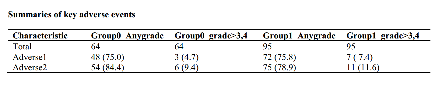
library("tableone")
###adverse event any grade, redefine a variable
dt$adverse1l<-ifelse(dt$adverse1>0,1,ifelse(dt$adverse1==0,0,NA))
dt$adverse2l<-ifelse(dt$adverse2>0,1,ifelse(dt$adverse2==0,0,NA))
listVars<-c("adverse1l","adverse2l")
table1 <- CreateCatTable(vars = listVars, data = dt, strata = "group",test=F)
table2 <- print(table1, showAllLevels = F,quote = F,varLabels = T)
table2<-as.data.frame(table2)
colnames(table2)<-c("Group0_Anygrade","Group1_Anygrade")
rownames(table2)<-c("Total","Adverse1","Adverse2")

###adverse event grade>3,4, redefine a variable
dt$adverse1h<-ifelse(dt$adverse1>2,1,ifelse(dt$adverse1<3,0,NA))
dt$adverse2h<-ifelse(dt$adverse2>2,1,ifelse(dt$adverse2<3,0,NA))
listVars<-c("adverse1h","adverse2h")
table3 <- CreateCatTable(vars = listVars, data = dt, strata = "group",test=F)
table4 <- print(table3, showAllLevels = F,quote = F,varLabels = T)
table4<-as.data.frame(table4)
colnames(table4)<-c("Group0_grade>3,4","Group1_grade>3,4")
rownames(table4)<-c("Total","Adverse1","Adverse2")

table5<-cbind(table2,table4)
table5<-table5[,c("Group0_Anygrade","Group0_grade>3,4","Group1_Anygrade","Group1_grade>3,4")]

# Write to RTF files
library(dplyr)
table5 <- table5 %>%
  mutate(Characteristic = rownames(.)) %>%
  select(Characteristic, everything()) %>%
  mutate_all(trimws)
library(rtf)
rtffile <- RTF("Summaries of key adverse events .rtf")
addHeader(rtffile, "Summaries of key adverse events ")
addTable(rtffile, table5, NA.string="")
done(rtffile)